![]()
![]()
![]()
![]()
![]()
![]()
Excerpt from:
Understanding the Federal Budget
Chapter 1: History of the National Debt
This eBook is available at Amazon.com for a $2.99 contribution to this website.
The federal deficit went from $74 billion in 1980 to $1.4 trillion in 2009 while the Gross National Debt went from $735 billion in 1980 to $16.7 trillion by the end of 2013. These numbers are truly mystifying to those of us who have never had to worry about a million dollars let alone a billion or a trillion. The purpose of this chapter is to put these numbers in perspective and to give them concrete meaning in terms of the magnitude of our federal deficit and debt problems.
Concepts and Definitions
We begin with a few basic concepts and definitions.
The Federal Deficit and National Debt
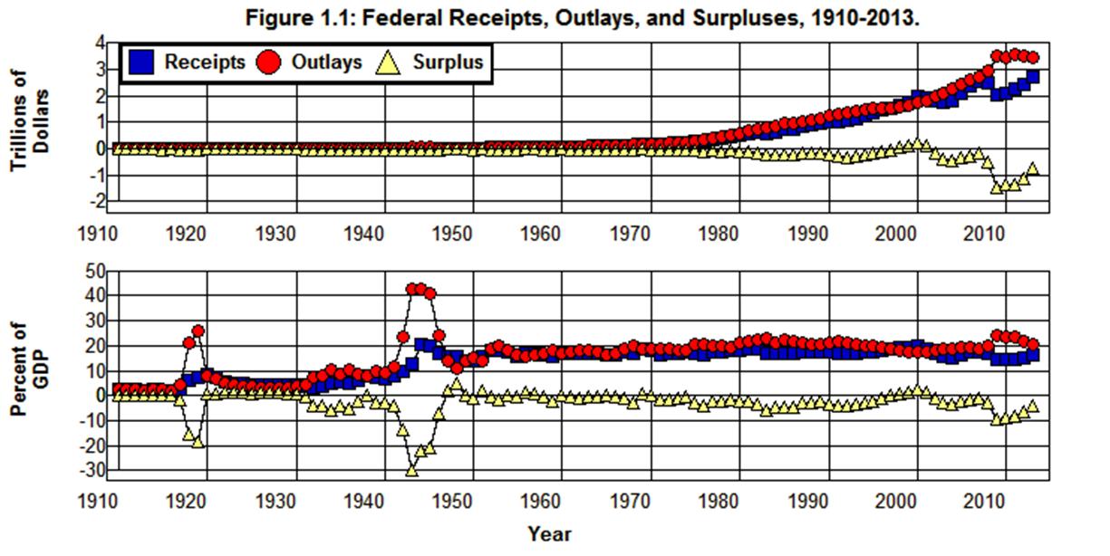
The difference between the amount of money the government takes in from taxes and other sources of revenue (its receipts) and the amount it pays out in purchases of goods and services and other kinds of expenditures (its expenditures or outlays) is officially called the surplus. When the government takes in less than it pays out this difference is negative, and this negative surplus is referred to as the deficit. The relationships between government receipts, expenditures, and its surpluses/deficits from 1910 through 2013 are shown in Figure 1.1, both in absolute amounts and as a percent of GDP. ource: Office of Management and Budget (1.1 1.2), Historical Statistics of the U.S. (Ca10) [2]
As can be seen in this figure, whenever the government’s Receipts are greater than its Outlays the Surplus is positive, and there is no deficit. Similarly, whenever the government’s Receipts are less than its Outlays the Surplus is negative, and a deficit results.
Federal surpluses and deficits are related to the national debt in that when the government takes in less than it pays out it must borrow the difference (equal to the deficit) to finance its excess expenditures. As a result, whenever there is a deficit the national debt increases by (approximately) the amount of the deficit. Similarly, whenever the government takes in more than it pays out the resulting surplus is positive and can be used to pay off the national debt. Thus, the national debt decreases by (approximately) the amount of the surplus. [3] One way of viewing the relationship between the national debt and the surplus/deficit is to think of the national debt as being the sum of all the deficits and surpluses the federal government has experienced since its inception.
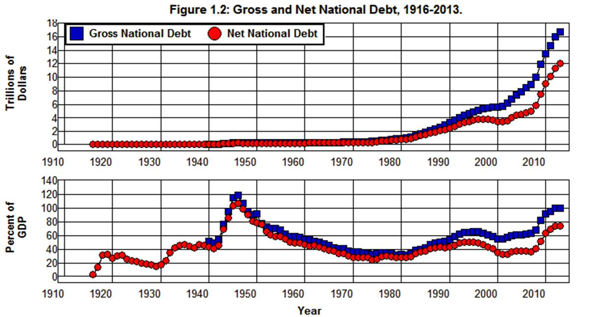
Figure 1.2 shows the total federal debt—commonly referred to as the National Debt—from 1916 through 2013, both in terms of absolute dollars and as a percent of Gross Domestic Product (GDP).
Source: Office of Management and Budget (7.1), Historical Statistics of the U.S.’s (Cj870) [4]
The federal debt is broken down into two categories in Figure 1.2:
The top line in Figure 1.2 plots the Gross National Debt, which includes all debt instruments issued by the federal government, including those held by federal agencies such as the Social Security Administration.
At the end of 2013 Gross National Debt stood at $16.7 trillion and Net National Debt at $12.0 trillion. Of the $4.7 trillion difference, $2.7 trillion was held by the Social Security Administration in its Old-Age Survivors and Disability Insurance (OASDI) trust fund with another $0.3 trillion in its Medicare Hospital Insurance (HI) and Supplementary Medical Insurance (SMI) trust funds—a total of $3.0 trillion. The remaining $1.7 trillion was in the combined holdings of all other federal government agencies. Throughout this eBook the terms “National Debt” and “federal debt” will refer to Net National Debt, unless designated otherwise.
Figure 1.1 is related to Figure 1.2 in that whenever the surplus is positive in Figure 1.1, the Net National Debt shown in the top half of Figure 1.2 decreases by (approximately) the amount of the surplus. Similarly, whenever the surplus is negative yielding a deficit in Figure 1.1, the Net National Debt shown in Figure 1.2 increases by (approximately) the amount of the deficit.[5]
Gross Domestic Product
As has been noted, the variables in the above figures are plotted both in terms of absolute values and as percentages of GDP. It should be obvious from looking at these figures that the absolute values do not tell us very much about the nature of our national debt problem. Judging by the plots of absolute values in Figure 1.1 and Figure 1.2 it would appear that there was no national debt or deficit problem during World War II. Just the opposite was true, of course, as is made clear by the fact that the Net National Debt had gone from 45% of GDP in 1940 to 106% of GDP by 1946.
In attempting to understand the federal budget as it relates to the economic system as a whole it is essential that the numbers be examined in relative terms, that is, in relation to some other variable in the economy. There are a number of ways this can be done, but, for present purposes, I will use GDP as the point of reference, and budget magnitudes will generally be expressed both in absolute terms and as a percent of GDP.
The reason for using GDP as the point of reference is that GDP is a measure of the total value of all goods and services produced in the domestic economic system, and as such, it gives us a measure of the size of our economy. It also represents the total gross income created in the process of producing domestic output in the economic system.[6] Total gross income is important to understanding the national debt because the national debt must be serviced—that is, the government must make both interest and principal payments on this debt. The ability of the government to service its debt without having to print money lies in its power to tax.[7] Since the main sources of the government’s tax revenues are from income and payroll taxes, the ratio of national debt to GDP (gross income) gives a measure of the relationship between the government’s debt and the tax base available to service its debt. In general, an increase in the debt to GDP ratio makes it more difficult for the government to service its debt; a decrease in the debt to GDP ratio makes it easier for the government to service its debt.
As for the government’s receipts, outlays, and surplus, just as with the national debt, the ratios of these entities to GDP give a rough measure of their relationship to the tax base on which they ultimately depend. As such, these ratios play a crucial role in determining the government’s ability to finance its expenditures from taxes.
It is also important to recognize that changes in the GDP will cause changes in government expenditures and receipts. Since GDP represents the total gross income earned in the economy, an increase in GDP will automatically increase the amount of money taken in by the government in the form of income, payroll, and other taxes. At the same time, it will tend to decrease the level of government expenditures as unemployment compensation, welfare, food stamps, and other governmental assistance expenditures fall. By the same token, a fall in GDP will not only cause tax receipts to fall, but will cause government expenditures to increase as government assistance and other emergency expenditures increase. Thus, a change in GDP will automatically affect the surplus or deficit as it affects government revenues and expenditures: An increase in GDP will automatically cause a surplus to increase or a deficit to decrease as tax receipts increase and expenditures fall; a decrease in GDP will automatically cause a surplus to decrease or a deficit to increase as tax receipts fall and expenditures increase. As a result, changes in GDP also affect the national debt.
The National Debt, 98 Years and Counting
Next we look to see how and why the national debt has changed since 1916.
World Wars, the Great Depression, and National Debt
The debt ratio rose from 2.7% of GDP in 1916 to 33% of GDP by 1919 as a result of World War I, but had fallen back to 16% of GDP by 1929. This feat was accomplished by keeping in place the personal and corporate income tax increases that were enacted to finance the war until they were reduced somewhat in1925.
At the beginning of the Great Depression the debt ratio rose again, this time to 46% of GDP by 1935. While it remained high during the 1930s, as a result of the Revenue Act of 1932 and other tax increase during the 1930s it remained fairly stable following 1935 and stood at 44% of GDP in 1940. Then came the deficits of World War II.
By today’s standards, government expenditures during the war were rather trivial in absolute terms, reaching a mere $92.7 billion in 1945. In relative terms they were huge, even by today’s standards, amounting to over 40% of GDP from 1943 through 1945. At the same time the deficit was also huge in relative terms. It reached 29.6% of GDP in 1943. The same is true of the national debt shown in Figure 1.2 which grew to $271 billion for the Gross National Debt and $242 billion for Net National Debt by 1946. This amounted to 119% and 106% of GDP, respectively.
The United States was saddled with a huge debt burden at the end of the war as measured by the size of its net debt relative to GDP, a burden that was systematically reduced over the following 29 years.
Falling Debt Burden from 1946 Through 1974
The federal budget was brought into balance fairly quickly after World War II, achieving a surplus in 1947. Though there were very few surpluses to follow, the budget was kept in fairly close balance from 1947 through 1974. As is shown in Figure 1.1, except for 1959 and 1968, the deficit was never greater than 2% of GDP. This fairly close balance allowed the debt to GDP ratio to fall, in spite of the deficits, because it meant that the rate at which the debt increased from 1947 through 1974 was less than the rate at which GDP increased during this period.
The primary mechanism by which the budget was brought under control was, as will be shown in Chapter 2, by cutting defense expenditures as a percent of GDP as other components of the government grew. At the same time, much of the wartime tax structure was kept in place: The top marginal income tax rate ranged from 92% to 70% during this period; the top marginal corporate profits tax rate ranged from 53% to 48%, and the top marginal estate tax rate was 77%. This tax structure made it possible for the government to raise the requisite revenue as the economy adjusted to the war’s end and as government expenditures grew throughout the 1950s and 1960s.
A secondary factor that contributed to reducing the debt burden was the policies of the Federal Reserve and Treasury. The Treasury dominated the Federal Reserve during and immediately following the war, a situation that continued until the 1951 Federal Reserve-Treasury Accord that gave the Federal Reserve a certain degree of independence. (Bernanke) The Treasury’s low interest rate policy preceding the Accord led to a substantial increase in the supply of money. This, in turn, led to an effective annual rate of inflation of 5.4% from 1946 through 1951, and a 33% increase in the average price level was the result.[8]
In the presence of a fairly balanced budget, the inflation that resulted from the Treasury’s low interest rate policy contributed greatly to reducing the burden of the debt. Low interest rates made it possible for the Treasury to refinance its debt as it came due at minimal costs while the inflation increased GDP relative to the debt. The effect was to cause the net debt to GDP ratio to fall from 106% in 1946 to 65% by 1951. This 38% (41 percentage point) decrease in the debt to GDP ratio was accomplished in spite of the fact that the real output of goods and services produced during that period increased by only 10%[9] and the actual debt fell by only 11%.
The rate of inflation was brought under control after the Accord, and the effective annual rate of inflation was a modest 1.9% from 1952 through 1967. The debt to GDP ratio continued to fall throughout this period even though the government continued to experience deficits in its budget. The reason is that the production of goods and services increased dramatically.
From 1952 through 1967 the output of goods and services produced in the United States increased at an effective annual rate of 3.4%. This led to a 78% increase in total output by 1967. When combined with the 1.9% effective annual rate of inflation and the resulting 32% increase in prices, the nominal value of GDP increased by 134% as Net National Debt increased by only 24%. The result was a fall in the debt to GDP ratio from 62% in 1951 to 31% by 1967. Thus, by 1967 the ratio of debt to GDP was below that of 1940, and the debt burden created by World War II had been completely eliminated[10] along with much of the burden created by the Great Depression.
The Kennedy-Johnson tax cuts combined with the escalation of the Vietnam War led to a deficit equal to 2.9% of GDP in 1968 that was converted into an 0.3% surplus in 1969 after the 1968 Revenue and Expenditure Control Act imposed a 10% income tax surcharge on individuals and corporations—the last surplus we were to see in the federal budget until 1998. The budget remained relatively balanced through 1974, and the debt ratio continued to fall with only a slight rise when the surcharge expired in 1970.
Debt Burden and the Great Inflation
From 1965 through 1984 we experienced what Alan Meltzer dubbed The Great Inflation. As was noted above, from 1952 through 1967 the effective annual rate of inflation was 1.9%. From 1967 through 1982 it was 6.6% and from 1975 through 1981 it was 7.7%. Unlike the 1945-1951 inflation, this inflation contributed relatively little to reducing the debt burden.
The 1973 Arab oil embargo with its concomitant quadrupling of the price of oil caused the economy to falter. The resulting 1973-1975 recession with its increase in unemployment equal to 3.6% of the labor force caused the deficit to increase in 1975 to 3.3% of GDP and to 4.1% of GDP in 1976 as the debt to GDP ratio increased from 23% in 1974 to 27% by 1977. This ratio then fell somewhat by 1981 and stood at 25% in at the end of that year.
The reason the inflation of the 1970s had relatively little effect on reducing the debt burden is that inflation can increase GDP relative to the debt only if inflation increases GDP sufficiently to offset the rate at which the deficit increases the debt. That didn’t happen in the 1970s. In fact, the effect of the inflation on the deficit made the deficit worse than it otherwise would have been, especially in the aftermath of the inflation.
Changes in prices have the effect of transferring purchasing power—that is, wealth—between borrowers and lenders. When prices rise over the period of a loan the money that is lent can purchase more goods and services than the money that is paid back. As a result, inflation has the effect of transferring wealth from lenders to borrowers. Similarly, when prices decrease over the period of a loan the money that is lent can purchase fewer goods and services than the money that is paid back. As a result, deflation has the effect of transferring wealth from borrowers to lenders. These transfers of wealth make the rate of interest at which people are willing to borrow or lend depend crucially on what they expect to happen to prices. Borrowers are less willing to borrow at high interest rates when they expect prices to fall and anticipate a loss in wealth from falling prices than when they expect prices to rise and anticipate a gain in wealth from increasing prices. The opposite is true for lenders; lenders are more willing to lend at low interest rates when they expect prices to fall and anticipate a gain in wealth from falling prices than when they expect prices to increase and anticipation a loss in wealth from increasing prices. As a result, inflationary expectations tend to lead to high interest rates, and deflationary expectations tend to lead to low interest rates.
No one expected the inflation that followed World War II. The greatest fear at the time was of recession and falling prices as had been the case at the end of previous wars. World War II broke that pattern, and before anyone realized it the lack of inflationary expectations on the part of borrowers and lenders made it possible for the Federal Reserve to maintain low interest rates during the inflation of 1945 through 1951. As a result, the Treasury was able to finance its deficits and rollover[11] its debt without adding significantly to the deficit.
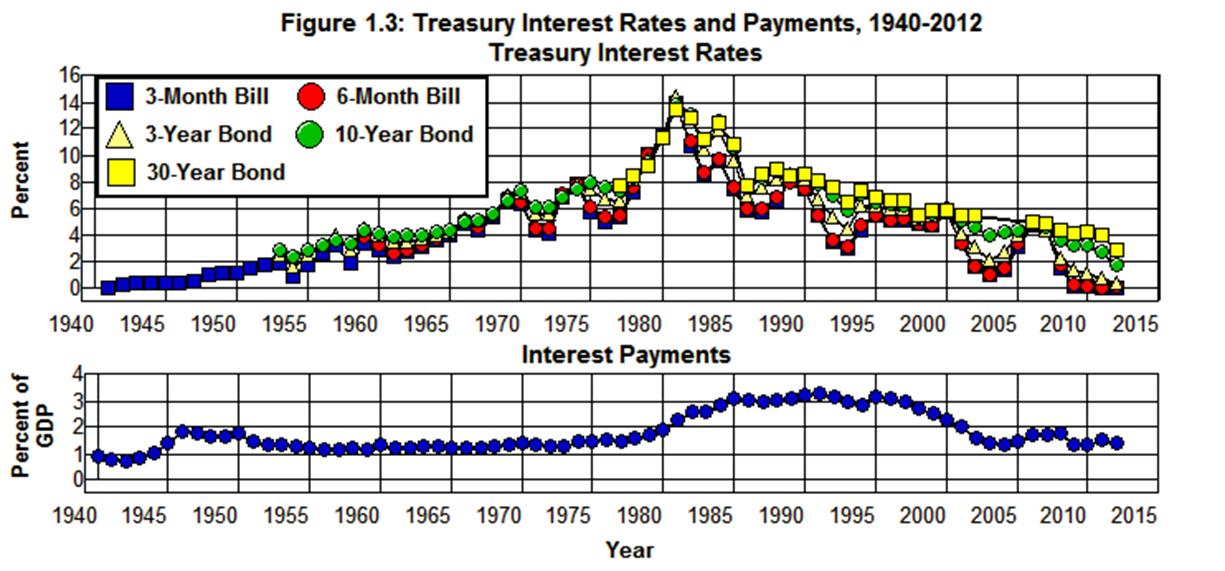
This was not the case during The Great Inflation with inflationary expectations rising throughout the period and remaining high into the 1990s. The effect of these rising and high expectations on interest rates can be seen in Figure 1.3 which shows the interest rates on various Treasury securities from 1941 through 2012.
Source: Economic Report of the President, 2012 (B73PDF|XLS), Office of Management and Budget. (3.1)
The spike in interest rates from 1979 through 1982 was obviously caused by the tight monetary policy of the Federal Reserve during that period, but interest rates remained high from 1975 through 1990 even when the Fed’s monetary policy was not tight. From 1975 through 1990, federal deficits had to be financed and the debt rolled over at long-term interest rates above 7% and short-term rates above 4% and often above 6%. The effect of having to rollover the debt at these exceptionally high interest rates is shown in Figure 1.3 by the dramatic increase in interest paid by the federal government on the national debt as a percent of GDP from 1975 through 1995.
From 1981 through 2010
The national debt rose dramatically following 1980, reaching a peak as a percent of GDP of 48% in 1993. This dramatic increase in debt was precipitated by the economic recession of 1981-1982 where unemployment increased by 3.9% of the labor force. When combined with the tax cuts in the Economic Recovery Tax Act of 1981 and the increase in national defense expenditures from 4.8% of GDP in 1980 to 5.9% in 1987 during Reagan’s anti-Soviet defense buildup, the result was soaring deficits that led to dramatic increases in the national debt.
The federal deficit averaged 0.39% of GDP in the 1950s. Aided by the Kennedy-Johnson tax cuts and the escalation of the Vietnam War, the average federal deficit increased to 0.76% of GDP in the 1960s, and, with the help of five additional legislative tax cuts in the 1970s, the average deficit increased to 2.0% of GDP in the 1970s. Then came the tax cuts in 1981 and the anti-Soviet defense buildup in the mid 980s, and the average deficit rose to 4.1% of GDP during the Reagan years.
These increases in deficits and debt were eventually brought under control by 1995, in spite of the 1990-1991 recession that increased unemployment by 2.2% of the labor force, and the debt ratio fell from 1996 through 2001. This was accomplished as a result of the Clinton tax increases in 1993 along with nine other relatively minor tax increases that were enacted following the 1981 tax cuts. There were also cuts in government expenditures from 1994 through 2000, mostly in defense following the end of the Cold War. A substantial increase in employment helped to reduce the deficit as well as the unemployment rate fell from 7.5% in 1992 to 4.0% in 2000. Net National Debt stood at $3.3 trillion in 2001 which was just 33% of GDP compared to the peak of 51% it had reached in 1994. In addition, there had been a surplus in the budget since 1998 which peaked at 2.3% of GDP in 2000.
Then came the 2001 recession, where unemployment increased by 2.0% of the labor force, and the 2001-2005 tax cuts, which led to a substantial loss in federal tax revenue. When combined with the increase in defense expenditures that accompanied the expansion of the war in Afghanistan into Iraq, the federal budget went from a surplus equal to 2.3% of GDP in 2000 to a 3.4% deficit in 2004, and the debt ratio went from 33% of GDP in 2001 to 37% in 2007. Then the housing bubble burst and unemployment began to increase.
The bursting of the housing bubble led to the 2007-2009 recession and an increase in unemployment equal to 5.0% of the labor force. In response, Congress passed the $152 Billion Economic Stimulus Act in February of 2008 to mitigate the effects of the economic downturn and the $700 billion Troubled Asset Relief Program (TARP) in October of that same year to bail out our financial institutions in the midst of the 2008 financial panic. Next came the $800 billion American Recovery and Reinvestment Act on February 17, 2009.
Net National Debt jumped from 37% of GDP in 2007 to 52% of GDP by the end of 2009 and, as a result of the financial crisis, the ensuing recession, and the efforts to stabilize the economy following the crisis, had risen to 74% of GDP by the end of 2013. As the government attempted to minimize the severity of the economic catastrophe that was unfolding in the wake of the housing bubble bursting the debt itself went from $5.0 trillion in 2007 to $12.0 trillion by the end of 2013—a 140% increase in just 6 years—as the deficit reached 9.8% of GDP in 2009 and then decreased to 4.1% of GDP by 2013 as a result of the economic recovery following 2009.[12]
Sequestration
In response to the rising federal debt, Congress passed the Budget Control Act of 2011 as a condition for increasing the debt ceiling in that year. This Act requires a $1.2 trillion reduction in federal discretionary spending over ten years, half of which is to come from cuts in defense expenditures and the other half from cuts in non-defense expenditures. This legislated reduction in discretionary spending (Sequestration) is approximately 25% of all discretionary spending in the federal budget, and Congress must decide whether to allow these arbitrary spending cuts to take place or whether to amend the law to keep this from happening. In the meantime, Congress is deadlocked over whether our deficit problem should be solved through tax increases or through expenditure cuts or some combination of the two, and, as was noted in the Prologue, the American people seem to want to solve the problem through expenditure cuts without actually cutting expenditures.
This brings us back to the question posed in the Prologue: Where are these cuts supposed to come from? The better part of valor would suggest that we first look to see how the money in the federal budget is actually spent and where it comes from before we attempt to answer this question.
Appendix on Output, Prices, and Productivity
This Appendix elaborates on of some of the more technical aspects of measuring total output and the average price level. It also examines the relationship between changes in GDP, productivity, and employment.
Measuring Output
GDP is the total value of all goods and services produced in the domestic economy. It is determined by multiplying the quantities of goods and services produced by their respective prices and summing to get the total value produced during a specific period of time. Thus, GDP measures the rate at which the total value of goods and services is produced. Since GDP is generally measured on an annual basis, it also tells us the total value of the goods and services that were produced in a given year. In addition, since the total value of goods and services produced corresponds to the gross income earned in producing those goods and services,[13] GDP also measures the rate at which total gross income is earned in the domestic economy and, when measured on an annual basis, the amount of gross income earned during a given year.
Employment is related to the quantities of goods and services produced, not their values as such. If we want a measure of total output that is related to total employment we must adjust the nominal or money value of GDP for changes in prices. This is normally done by choosing the prices that exist at a particular point in time (or averages of prices over a particular period of time) and using those prices to measure the value of the output of goods and serves produced at other points in time. When the value of GDP is measured in this way the result is referred to as real GDP or GDP in constant prices, base year prices, or in base year dollars. Since real GDP is measured by holding prices constant, changes in real GDP can occur only if quantities change. Hence, real GDP gives us a way to measure changes in the sum of all the quantities of output produced.
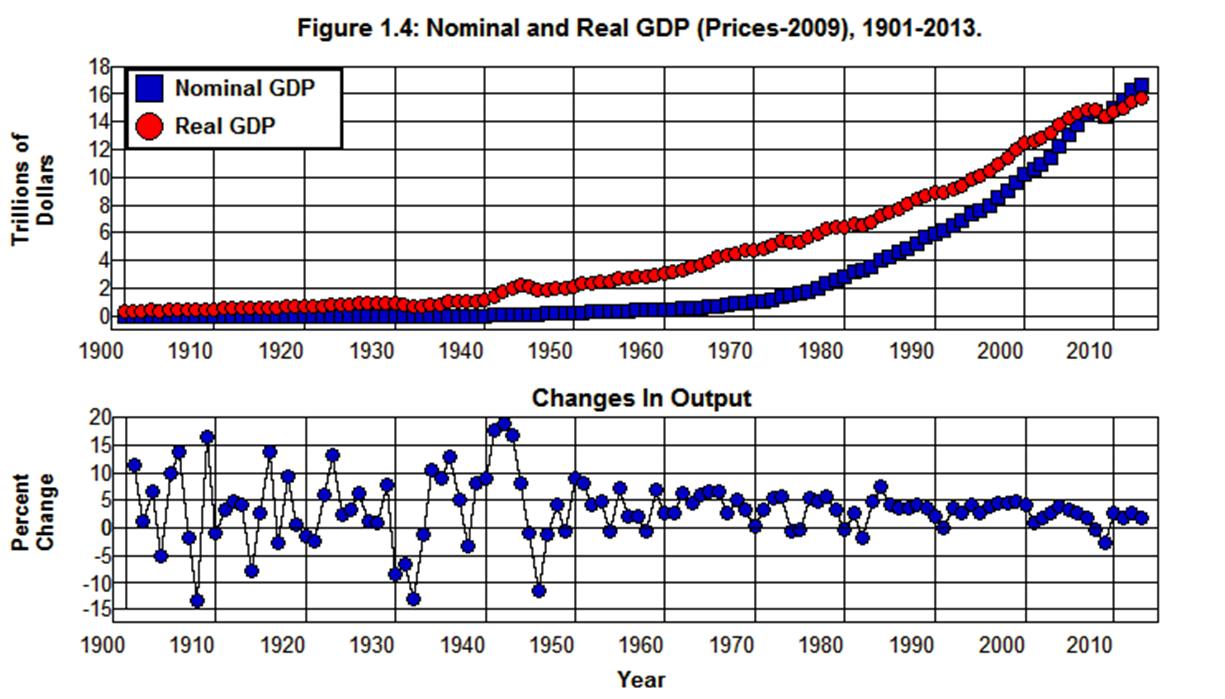
Nominal GDP and Real GDP measured in 2009 prices are plotted in Figure 1.4 from 1901 through 2013 using data from the Historical Statistics of the U.S. (Ca9, Ca10) for the years 1901 through 1928 and from the Bureau of Economic Analysis (1.1.5 1.1.6) for the years 1929 through 2010. Nominal GDP and Real GDP in Figure 1.4 are, of course, the same in 2009 since that is the base year—the year from which the prices used to measure the value of the output produced in all of the years were obtained.
Source: Bureau of Economic Analysis. (1.1.5 1.1.6) Historical Statistics of the U.S. (Ca9, Ca10)
The values of Nominal GDP are below those of Real GDP in the years preceding 2009 in Figure 1.4 because prices in those years were, on average, lower than they were in 2009. As a result, the value of Nominal GDP measured in current prices—that is, in prices that existed at the time—in those years underestimate the differences in the total quantity of output produced relative to that produced in 2009. Similarly, the values of Nominal GDP are above those of Real GDP in the years following 2009 because prices in those years were, on average, higher than they were in 2009. As a result, the value of Nominal GDP in those years overestimate the differences in total quantity of output produced relative to that produced in 2009.[14]
The year to year percentage changes in Real GDP are also plotted in Figure 1.4 (Changes in Output). These rates of change give us a measure of the rates as which aggregate (i.e., total) output changed from year to year.
Finally, it should be noted that what we are doing here is adding apples and oranges which, of course, everybody knows you can't do. But the fact is, you can add apples and oranges if you have a common unit of measurement, such as pounds or bushels. It is important to remember, however, that when you do this you don't end up with either apples or oranges, but, rather, pounds or bushels of fruit, and the sum tells us nothing at all about the kind of fruit that is included in the result. In measuring the total output produced within the economy, the common unit of measurement is the monetary unit, dollars, and the result of summing the various outputs of goods and services produced as measured in dollars is the total value of output produced—the real value if prices are held constant over time or the current or nominal value if the prices that are current at the time are used. In either case, the sum tells us nothing at all about the composition of the total or how the composition changes over time. It only tells us the value of the output produced. This apples and oranges problem is intrinsic in all aggregate measures (measures arrived at by adding to obtain a total) of disparate economic variables.[15]
Measuring Prices
Since the difference between the value of nominal GDP and real GDP in each year is caused by the differences between current year prices and the prices that existed in the base year (2009 in Figure 1.4), if we divide nominal GDP by real GDP and multiply by 100 the result is a price index that expresses the weighted average (weighted by current year quantities produced) of current year prices to base year prices as a percent of base year prices. This index is called the Implicit GDP Deflator. A measure of the rate of inflation that includes all goods and services that are produced within the economic system can be obtained from this index by calculating its year to year percentage changes.
The Implicit GDP Deflator in 2009 prices is plotted from 1900 through 2013 in Figure 1.5 using the GDP deflator implicit in the Historical Statistics of the U.S. (Ca10) for the years 1900 through 1928 and in the series published by the Bureau of Economic Analysis (1.1.5) for the years 1929 through 2013. The year to year percentage changes in this index that give the rate of inflation—that is, the rate of change in the average price as measured by the index—for each year is also plotted in this figure.
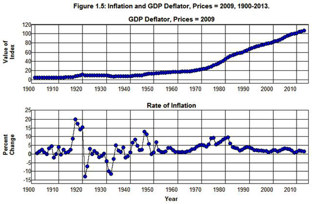
Source: Bureau of Economic Analysis. (1.1.5) Historical Statistics of the U.S. (Ca10)
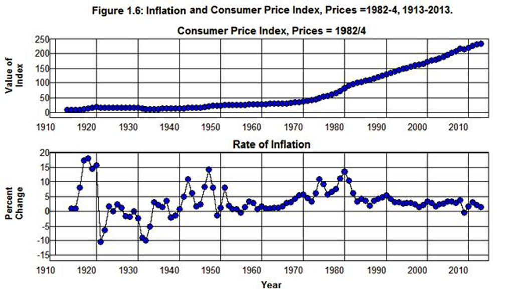
While the Implicit GDP Deflator provides a measure of the average price level of all goods and services produced in the economic system, the Consumer Price Index (CPI) provides a measure of the average price level of those goods and services that consumers purchase. It is constructed by surveying consumers to determine how they spend their incomes and creating a representative market basket that contains goods and services in proportion to the averages of the goods and services purchased by the consumers surveyed. Since the quantities in this market basket are fixed, and value of this market basket changes as prices change over time, if we divide the value of the market basket in each year by the value of the market basket in some base year and multiply by 100, the result is an index that expresses the weighted average (weighted by the quantities in the representative market basket) of current year prices to base year prices as a percent of base year prices. A measure of the rate of inflation as it affects consumers can be obtained from this index by calculating its year to year percentage changes.
The Consumer Price Index (which uses the average value of the market basket for the period from1982 through 1984 for the base year) is plotted from 1913 through 2013 in Figure 1.6. The year to year percentage changes in this index are also plotted in this figure.
Source: Bureau of Labor Statistics.
Output, Productivity, and Employment
We can use real GDP as a measure of the output of goods and services produced in the economy, and by taking the year to year percentage change in this measure we can calculate the rate at which total output increases or decreases in each year. These rates are plotted in the bottom graph in Figure 1.4. They are important because the level of employment over time depends, in part, on the quantity of output produced. In general, an increase in the quantity of output produced is associated with an increase in employment and a decrease in the quantity of output produced is associated with a decrease in employment. However, the level of employment not only depends on the quantity of output produced, it also depends on the way in which output is produced.
The reason is that the amounts and kinds of tools and equipment and the ways things are done tend to increase and improve over time. These increases in the capital stock (tools and equipment) and improvements in technology (ways of doing things) tend to increase the productivity of labor over time which means they increase the amount of output a given number of workers can produce during a given amount of time. As a result, in order to maintain a given level of employment, real GDP must increase over time at the rate labor productivity increases. By the same token, in order to increase the level of employment real GDP must increase at a rate that is greater than the rate at which labor productivity increases.
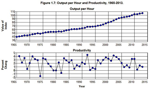
The Bureau of Labor Statistics’ productivity index of output per hour is plotted in Figure 1.7 from 1965 through 2013 along with the percentage changes in this index. The percentage changes in this index give the year to year rates at which labor productivity changed during each year.
Source: Economic Report of the President, 2014. (B49PDF|XLS)
From 1965 through 2013 this index increased from 39.4 to 106.2 which implies an effective annual rate of increase equal to 2.1% per year. This means that real GDP had to increase, on average, by 2.1% per year over the previous 48 years just to maintain the level of employment that existed in 1965. It also means that during those 48 years it was necessary for output to grow, on average, by 2.1% plus the rate at which the labor force grew in order to keep the labor force fully employed.
Endnotes
[2] Until 1976 the federal government’s fiscal year began on July 1 of the previous calendar year. Since 1977 the federal government’s fiscal year has begun on October 1 of the previous calendar year. The Office of Management and Budget (OMB's) data as a percent of GDP only go back to 1930 and correspond to the federal government's fiscal year rather than the calendar year. Unfortunately, the OMB does not provide fiscal year GDP estimates for the years before 1930. I use the OMB's estimates for fiscal year GDP throughout this paper when looking at budget data, except for the years before 1930. For the years before 1930 I use the mean of the current and previous calendar years' GDP from the Historical Statistics of the U.S. (Ca10) to estimate the fiscal year value of GDP and divide this value into the OMB’s fiscal year nominal values in its various tables to obtain the fiscal year percentages of GDP. Using this methodology, the data from Historical Statistics yields results that are identical, except for rounding error, to the OMB’s fiscal year estimates of GDP for the years in which these two series overlap.
[3] This relationship is not exact in that the government can borrow money it doesn’t spend, thereby increasing the amount of cash it holds rather than paying down debt, and it can spend money in excess of its revenue without borrowing by reducing its holdings of cash. The government can also affect its cash/debt holdings by buying and selling assets that are, by definition, not included in its expenditures or revenue. See the Bureau of Economic Analysis's Table 3.2 for a discussion of this aspect of the budgeting process.
[4] The series on National Debt published in the Office of Management and Budget’s Table 7.1 only goes back to 1940. The estimates for Net National Debt prior to 1940 are taken from the Historical Statistics of the U.S.’s Cj870 which gives estimates for Federal Public Debt back to 1916. Unfortunately, Historical Statistics of the U.S.’s does not give estimates for Gross National Debt so Figure 1.2 does not contain estimates for Gross National Debt prior to 1940, only for Net National Debt. It must also be noted that Federal Public Debt in Historical Statistics does not correspond exactly to the OMB’s Net National Debt in that the Historical Statistics estimates are on a calendar year basis and the OMB’s estimates are on a fiscal year basis. (See footnote 2 above.)
[5] See footnote 3 for the qualifications to this rule.
[6] In addition, GDP is related to the total levels of output produced and employment as well as to the level of total gross income. Some of the more technical concepts relating to GDP, employment, output, and income are explained in the Appendix at the end of this chapter.
[7] The federal government also has the ability service its debt by printing money. The important and limitations of this fact are discussed in A Note on Managing the Federal Budget and in Where Did All The Money Go?
[8] These effective annual rates of inflation, as well as those that follow, are calculated from the 2009 base year GDP (chained) Price Index published by OMB in Table 10.1. The effective annual rates used throughout this paper are calculated from the compound interest formula:
Pn = P0 x ∏(1 + r)i,
where
i = 0, 1, 2,. . .,n,
P0 is the starting principle,
Pn is the ending principle, and
r is the effective annual rate.
This formula assumes annual rather than continuous compounding. (See the Appendix at the end of this chapter for a discussion of price indices.)
[9] This value was computed by deflating OMB’s fiscal year GDP in Table 0.1 by the 2009 base year GDP (chained) Price Index in this table and calculating the percentage change in the resulting real value of GDP measured in 2009 prices from 1945 through 1951. Changes in fiscal year output will be measured in this way in what follows. (See the Appendix at the end of this chapter.)
[10] The debt ratio actually fell below its 1940 level in 1962.
[11] Approximately one third of the national debt is in the form of Treasury bills that mature in less than one year and one half is in the form of Treasury notes that mature in less than ten years. (B87PDF-XLS) When there is a deficit in the federal budget, the debt obligations of the government must be paid when they come due by the government issuing new debt instruments in order to obtain the cash necessary to pay off the old debt instruments—that is, the Treasury must rollover its debt.
[12] See Where Did All The Money Go? for a comprehensive analysis of the events leading up to the financial crisis of 2008 and the fallout from that crisis.
[13] Since the profit earned by the owners of a business is defined as the value of goods and services produced by the business less the incomes paid out by the business to others in the process of producing goods and services, when we add total profits to all of the other kinds of income earned in producing the total output to get total income, the result is equal to the value of total output. Thus, given the residual nature of profits in the national income accounting system, the value of total output is by definition equal to the value of output produced.