Real-World
Economics

 

Simulating the CBO’s Budget
Projection Scenarios

George H. Blackford © 1/31/2014

The Congressional Budget Office (CBO) publishes an annual report that provides projections for the federal budget under two scenarios: an extended baseline scenario and an extended alternative fiscal scenario.  According to the CBO:

The extended baseline scenario generally adheres closely to current law. . . .

 

Under . . . the extended alternative fiscal scenario, certain policies that are now in place but that are scheduled to change under current law would continue instead, and some provisions of current law that might be difficult to sustain for a long period would be modified. . . . The 2013 Long-Term Budget Outlook.

 

Given these scenarios, the CBO projects federal spending and revenue over specific periods of time to show how these projected levels of revenues and spending can be expected to affect federal debt in the future.

Simulating the CBO’s Projection Models

The simplest way to construct a model that simulates the underlying models that generate the CBO’s projections is to assume that federal debt at the end of the current year (D_i) will be equal to a) the debt at the end of the previous year (D_i-1) plus b) the interest paid out during the current year (I_i) plus c) the non-interest expenditures paid out during the current year (NIS_i) less d) the revenues collected during the year (R_i):

1)  D_i = D_i-1 + I_i + NIS_i - R_i.

This relationship is not exact in that it does not take into account changes in the cash holdings of the federal government, the accumulation or sale of assets, or the way in which other factors affect federal borrowing that are not included in the budget. Nevertheless, equation 3) can be used to define a model that approximates the effects of changes in the OMB's revenue and spending projections by specifying:

2)  I_i = r_iD_i-1 + r_i(R_i - NIS_i)/2

        = r_i / (D_i-1 + (R_i - NIS_i)/2),

where r_i is, in effect, the average rate of interest paid on the federal government’s debt and borrowings during the year; (R_i - NIS_i) is the amount of money during the current year that the government may have to borrow to fund its expenditures or that is available to the government to pay back debt (dividing by 2 presumes that money is borrowed or paid back at a constant rate throughout the year); and the other variables are as defined in equation 1).  

The significance of 2) is that it can be solved for r_i,

3)  r_i = I_i / (D_i-1 + (R_i - NIS_i)/2),

and, given the values for D_i, R_i, and I_i in the Supplementary Data Excel workbook that is published with the CBO's reports, equation 3) can be used to estimate the values of r_i that are implicit in the CBO's projection models.  These estimates can, in turn, be used with equation 2) to estimate the value for I_i for any set of values for D_i-1, R_i, and NIS_i.  These estimated values for I_i can then be substitute into 1) to obtain the corresponding values for D_i.  Thus, equations 1) through 3) allow us to approximate how changes in the values of non-interest spending and revenues will affect the CBO’s projections. 

Using Excel to Simulate the CBO’s Projection Models

I have incorporated the simulation model specified in 1) through 3) above in an Excel workbook that can be downloaded by clicking on this link. This workbook contains five spreadsheets: Baseline Data, Alternative Data, Baseline Simulation, Alternative Simulation, and Historical Data.  These spreadsheets are saved in a protected mode without a password so they can be unprotected to play with the formulas at your discretion. 

Baseline Data Spreadsheet

The first N Columns of the Baseline Data spreadsheet are copied from the 1. Summary Extended Baseline spreadsheet in the Supplementary Data workbook. The Real GDP 2013 Prices and Nominal GDP variables in Column P and Column Q are copied from the 2. Economic Vars and Population spreadsheet in the Supplementary Data workbook that accompanied the CBO’s 2013 report.  These last two variables are used to calculate the Implicit GDP Deflator in Column R by dividing Column Q by Column P. (You’ll have to ask the CBO why the result equals 0.99 in 2013 rather than 1.00.) 

Equation 3) is used to estimate the Average Rate of Interest parameters (r_i) in Column T of the Baseline Data spreadsheet using the values for Revenues (R_i) in Column B, Net Interest (I_i) in Column H, and the Calculated Debt/GDP (D_i-1) in Column V where D_i is calculated using equation 1) and the ith values of the independent variables in 1).  The value for D₂₀₁₂ is obtained from Column C of the Historical Tables spreadsheet in this workbook. The value for total non-interest spending (NIS_i) in 1) through 3) is calculated from the sum of Columns C through F, rather than being obtained directly from Total Noninterest Spending in Column G, to keep the calculation of the r_i parameters consistent with the way in which these parameters are used in the Baseline Simulation spreadsheet, thereby, minimizing the rounding error in the calculations.

The CBO does not provide projections for defense expenditures, the second largest component of the federal budget after Social Security, but because of its importance in the federal budget I have attempted to separate out Defense in Column S in this spreadsheet from the Other category in Column F in the CBO’s data base. In doing this I have used the Office of Management and Budget's estimates for defense expenditures in its Table 3.1 for the years 2013 through 2018 and have assumed that defense expenditures remain a constant proportion of the CBO's projections for all Other non-interest spending thereafter.   This treatment of defense seems to be in accord with the CBO's discussion of discretionary spending of which defense expenditures are the largest component. 

Finally, it should be noted that since the CBO reports all of its projections as a percent of GDP (Gross Domestic Product), almost all of the calculations in this spreadsheet (and throughout the rest of this workbook) require that the various percentages be multiplied by the corresponding value of GDP in Column Q to obtain their absolute magnitudes before the calculations in 1) through 3) can be made and then divided by the corresponding values of GDP to convert the results back to percentages of GDP.

Alternative Data Spreadsheet

The Alternative Data spreadsheet is identical to the Baseline Data spreadsheet explained above except that the first N columns of the Alternative Data spreadsheet are copied from the 6. Summary Ext Alt Fiscal Scen spreadsheet in the Supplementary Data workbook rather than from the 1. Summary Extended Baseline spreadsheet.

Baseline Simulation Spreadsheet

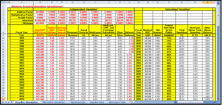
As is shown in Figure 1, the Baseline Simulation spreadsheet is broken down into two sections: Independent Variables and Calculated Variables. 

Figure 1: Baseline Simulation Spreadsheet

The subsection at the top of the Independent Variables section allows you to enter values in the Additive Factor (AF), Multiplicative Factor (MF), Growth Factor (GF), Maximum (Max), and Minimum (Min) rows that are used to transform the variables (Var_i) (all of which are taken from the various columns of the Baseline Data spreadsheet) in the corresponding columns below this subsection.  These transformations are calculated according to the formula:

4)       Var_i* = Min < AF + MF×Var_i + (GF≠0)×Var_i×(1+GF)^{(Current Year-2013)} < Max.

The transformed variables (Var_i*) are then used in conjunction with equations 1) through 3) above and the r_i parameters calculated in the Baseline Data spreadsheet to calculate the variables in the Calculated Variables section of the spreadsheet, beginning in 2014, to show how the transformed independent variables will affect the projections of Nominal GDP, Net-Interest, Federal Debt Held by the Public, Total Spending, Revenues Minus Total Spending, and Other Minus Defense in the CBO’s extended baseline scenario projection model.

Alternative Simulation

The Alternative Simulation spreadsheet is identical to the Baseline Simulation spreadsheet except the independent variables in the Alternative Simulation spreadsheet are taken from the Alternative Data spreadsheet rather than from the Baseline Data spreadsheet.

Historical Data

The Historical Data spreadsheet combines the projection and transformed data from 2013 through 2088 in the other spreadsheets in this workbook with the historical data from 1950 through 2012 for these data.  The locked cells in this spreadsheet can be copied and passed into other programs.

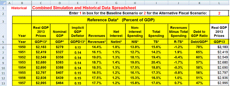
As is shown in Figure 2, at the top of this spreadsheet is a selection box. 

Figure 2: Historical Data Spreadsheet.

This box is used to select whether the projection data from the baseline scenario or the alternative fiscal scenario spreadsheets are to be combined with the historical data.  Entering a 1 in this box will combine the historical data with the data in the Baseline Data and the Baseline Simulation spreadsheets; entering a 2 in this box will combine the historical data with the data in the Alternate Data and Alternate Simulation spreadsheets.

The Historical Data spreadsheet is broken down into four sections: Reference Data, Independent Variables, Calculated Variables, and Summary Table. 

The Reference Data section combines historical data with the untransformed projection data from the Data spreadsheet of the scenario that has been selected. 

The Independent Variables section combines historical data with the transformed independent variable data from Simulation spreadsheet of the scenario that has been selected. 

The Calculated Variables section combines the historical data with the calculated variable data from the scenario that has been selected and also calculates a number of additional variables that are projected in the CBO’s projection models that are not calculated in the simulation spreadsheets: Revenues Minus Total Noninterest Spending, Total Spending, Revenues Minus Total Spending, Social Security Plus Medicare, Social Security Plus Healthcare, Other Excluding Defense, and Total Healthcare.

The Summary Table section displays the transformation parameters entered in the Simulation spreadsheet of the scenario that has been selected and also summarizes the changes in the most important projected variables between 2013 and 2038, 2049, and 2088 which are reference points used in the CBO’s 2013 report.  These changes are also displayed at the bottom of the other three sections of the Historical Data spreadsheet (and at the bottom of the tables in the Baseline Simulation and Alternative Simulation spreadsheets as well) for all of the variables in this spreadsheet.

Model Accuracy

There is not enough data in the CBO’s Supplementary Data workbook to check the accuracy of this model directly, but there are two ways to evaluate its accuracy indirectly.  The first is to see how well the estimates produced by the model forecast the data from which the r_i parameters of the model are derived. 

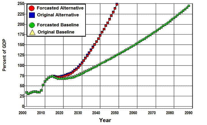
Figure 3 plots the original values of the CBO’s 2013 baseline and alternative fiscal scenario projections and the model’s estimates of these projections. 

Figure 3: Comparing Baseline and Alternative Fiscal
Projections and Forecasted Values.

The fit is quite good, though there is some autocorrelation indicated by the way in which the forecasts seem to lag the changes.  The mean error is -0.98 percentage points in the baseline forecasts with a standard deviation of 1.02, while the mean error is -1.24 percentage points for the alternative forecasts with a standard deviation of 0.77.  The mean absolute error for the baseline forecasts is 1.09 percentage points with a standard deviation of 0.91, and is 1.27 percentage points for the alternative fiscal forecasts with a standard deviation of 0.77. 

These numbers suggest that the model works quite well within the data on which it was estimated, but this does not tell us very much about its accuracy outside this data. 

The second way we can evaluate the accuracy of this model is to look at the accuracy with which it forecasts the fiscal gaps that the CBO publishes in its reports:

The fiscal gap is a measure of the difference between projected federal noninterest spending and revenues over a given period.  It represents the extent to which the government would need to immediately and permanently raise tax revenues or cut spending—or do both, to some degree—to make the government’s debt the same size (relative to gross domestic product) at the end of the period that it is at the end of 2013.  The 2013 Long-Term Budget Outlook

The CBO specifies three fiscal gaps for its baseline scenario in its 2013 report for the periods: 2013-2038, 2013-63, and 2013-2088.  In its 2012 report also specifies fiscal gaps under its baseline scenario for the periods 2012-2037, 2012-2062, and 2012-2087 along with a fiscal gap under its alternative fiscal scenario for the period 2012-2037. 

Each of these gaps can be converted to a revenue gap and a spending gap—that is, the amount by which revenue or spending must permanently increase or decrease in order to eliminate the fiscal gap—by dividing the CBO’s fiscal gap, which is expressed as a percent of GDP, by the CBO’s projected levels of revenue and spending in the second year of the period, which is also expressed as a percent of GDP.   This is done in Table 1 which shows the CBO’s fiscal, revenue, and spending gaps from the CBO’s 2013 and 2012 reports.

Table 1: The CBO's Fiscal, Revenue, and Spending Gaps, 1913 and 1912.
	2013 Baseline Scenario
Period	Fiscal Gap	2014 Revenue	Revenue Gap	2014 Spending	Spending Gap
2014 to 2038	0.90%	17.7%	5.1%	19.5%	4.6%
2014 to 2063	1.40%	17.7%	7.9%	19.5%	7.2%
2014 to 2088	1.70%	17.7%	9.6%	19.5%	8.7%
	2012 Baseline Scenario
Period	Fiscal Gap	2014 Revenue	Revenue Gap	2014 Spending	Spending Gap
2012 to 2037	-0.80%	18.7%	-4.3%	21.0%	-3.8%
2012 to 2062	-1.00%	18.7%	-5.3%	21.0%	-4.8%
2012 to 2087	-1.10%	18.7%	-5.9%	21.0%	-5.2%
	2012 Alternative Fiscal Scenario
Period	Fiscal Gap	2014 Revenue	Revenue Gap	2014 Spending	Spending Gap
2012 to 2037	4.60%	16.7%	27.5%	21.5%	21.4%

The revenue and spending gaps in Table 1 are compared with the simulation model’s estimates of these gaps in Table 2.

Table 2: Comparing the Model's Estimates with the CBO's Projections of Fiscal Gaps.
	Baseline Revenue Gaps, 2013				Baseline Spending Gaps, 2013
Period	Model	CBO	Diff.	%	Model	CBO	Diff.	%
2013-38	5.0%	5.1%	0.05%	1.1%	-4.8%	-4.6%	0.19%	-4.1%
2013-63	7.6%	7.9%	0.34%	4.3%	-7.1%	-7.2%	-0.04%	0.5%
2013-88	8.5%	9.6%	1.08%	11.3%	-8.0%	-8.7%	-0.73%	8.4%
	Baseline Revenue Gaps, 2012				Baseline Spending Gaps, 2012
Period	Model	CBO	Diff.	%	Model	CBO	Diff.	%
2012-37	-3.9%	-4.3%	-0.38%	8.8%	4.1%	3.8%	-0.25%	-6.5%
2012-62	-4.3%	-5.3%	-1.02%	19.1%	4.6%	4.8%	0.19%	3.9%
2012-87	-4.4%	-4.9%	-0.47%	9.6%	4.7%	5.2%	0.56%	10.6%
	Alternative Fiscal Revenue Gaps, 2012				Alternative Fiscal Spending Gaps, 2012
Period	Model	CBO	Diff.	%	Model	CBO	Diff.	%
2012-37	25.3%	27.5%	2.23%	8.1%	-20.2%	-21.4%	-1.16%	5.4%
Summary
			Revenue Gaps		Spending Gaps		Combined
Mean Error			0.26%		-0.18%		0.04%
Std. Dev.			1.09%		0.59%		0.87%
Mean Absolute Error			0.80%		0.44%		0.62%
Std. Dev.			0.73%		0.40%		0.59%

Here we find a mean error for the fourteen-gaps estimated to be 0.04 percentage points with a standard deviation of 0.87, and an absolute mean error of 0.62 percentage points with a standard deviation of 0.59. 

When we separate the revenue and spending gaps we find there is are somewhat larger mean errors and standard deviations for revenue gap forecasts than for spending gap forecasts, 0.26 versus -0.18 for the mean error and 0.8 versus 0.44 for the mean absolute error.  

These numbers suggest it is reasonable to assume the model is accurate in estimating the revenue and spending gaps within eight or ten percent of the CBO’s projections, though there is one obvious outlier in the estimate of the CBO’s 2012-2062 baseline scenario revenue gap.